April 14th Module
Wellness Rollcall!
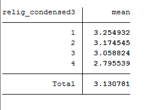
Let’s remind ourselves how we recoded the religion variable:
relig_condensed:1 - Non-Catholic Christianity2 - Catholicism3 - Non-Christian, but Religious4 - No Religion
We can see four groups (Non-Catholic Christian, Catholic, Non-Christian Religious, and Not-Religious)
What the ANOVA test allows us to do is find out if there is a statistically significant difference in means between groups.
Now we can orient to where we stopped last week…
We were using ANOVA to test the Null Hypothesis is that all the group means are equal to one another. In this case, that Catholics, Non-Catholic Christians, Religious Non-Christians, and Non-religous people all have the same mean ideal number of children.
So we ran our One-Way ANOVA test in Stata.
Look at all the work it did for you! And some familiar friends are here! You have the F-statistic, your within and between group variances, some degrees of freedom! And our old pal, the p-value which is all the way to the right there under “Prob>F”. This is the most important element of the output. If this value is less than .05 we can reject our null hypothesis. And it is! So we can!
We can reject the null hypothesis that all the groups have the same mean.
Let’s consider how this is different than what a T-Test would allow.
In this week’s activity, you’ll have the opportunity to use both t-tests and ANOVA testing to address the above questions. Start to develop an intuition for when and why one test might be more valuable or more appropriate than another.
Two-Way ANOVA Testing
What you’ve done so far of ANOVA testing is “one-way” ANOVA testing. But you can actually layer on additional grouping variables, once you understand the basic logic. Let’s consider some other variables from my list.
chldidel sexraceImagine I wanted to look at differences in sex categories and differences in race categories. I could run a two-way ANOVA test. And the syntax in Stata is incredibly simple. Just put your “dependent variable” (your interval-ratio variable) first.
Look at those p-values in the far right column. Remember, you’re looking for significance at the p<.05 level. You can see that sex qualifies for statistical significance, and race does not.
You might be wondering…
why you wouldn’t simply run two separate ANOVA tests, one for sex and one for race. The multivariate ANOVA test doesn’t simply run separate evaluations of each grouping variable. They produce a single model based on all the variables incorporated. So we can observe how the variables work together.
Check this out…
Below is a two-way ANOVA test of income and race. You can see in the far right column that we just barely have significance at the p<.05 level. So we would say based on this test that there is a statistically significant difference in income between racial groups.
But look at this…
When we add “education” to our model, and the model “accounts” for the within and between variance of both race and education, the significance of the race variable “drops out.” It’s jumped to a p-value of .23, while education remains significant.
We won’t do much with this in this course, but this logic will be incredibly important to any statistics work you do in the future. It is this logic that allows sociologists who are examining the relationship between to variables, to “control for” or “account for” the “influence” of other variables on the relevant outcomes. This week (and next) you’ll try this on with your own variables.
Summary: What you need to know of ANOVA testing for the purposes of this course is:
One-way ANOVA testing allows us to consider differences across more than two groups within a variable
Two-way ANOVA testing allows us to consider more than one grouping variable
ANOVA testing requires that your “dependent variable” is interval-ratio level and continuous
ANOVA testing assumes approximate normality in your dependent variable for each of the groups, homogeneity between variables (you don’t need to know what that means yet, but if you still have your book you’ve read a bit on this), and that there are no major outliers. (You aren’t required to do these checks for your portfolio, but it’s good to know for “the real world”)
What ANOVA testing is examining is how much variation on a dependent variable can be “explained” by within-group variance, and how much can be “explained” by between-group variance, for each independent variable.
You’ll play with this a bit in our last weekly activity.
One… More… Technique!
Team this is so exciting. You only have one more technique to learn. And it’s Linear Regression (we will sometimes call this OLS regression which stands for “ordinary least squares” regression). And the thing that’s cool about this is that you already understand the logic of linear regression… because you went to middle school… and you learned what a slope was… Ok let’s time travel for a second…
Remember this?
y = mx + bOf course you do. And for some of you this brings up powerful feelings of accomplishable SAT questions. For others it yields only fear. All reactions are welcome.
But this should also look familiar:
Now here’s a fun fact:
Remember when we did correlations to examine effect size? Let’s stick with “education” and “income” and look at one.
And you would look at that and say “Wow. What a lovely, direct, moderate effect size we have there between education and income! Another way to think about this “effect size” is that it’s a kind of slope. That’s essentially what a correlation coefficient is. The “m” in the “y=mx+b” formula, is a correlation coefficient, telling you how “y” correlates with “x.”
Now imagine you’re interested in the relationship between education and work hours. We are interested in the correlation between years of education and weekly work hours. These are both ratio level variables in the GSS…
But it’s still middle school…
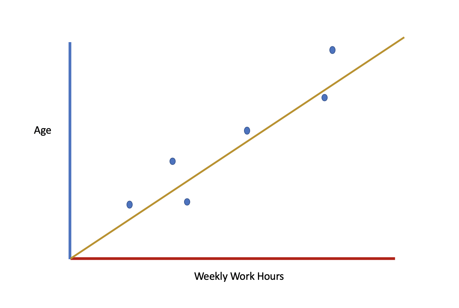
You’d be like “Hey Miss J, look at this X & Y axis situation representing age and weekly work hours!” and your teacher would be like “Wow! Great job!”
And then she’d be like “Can you chart the line of best fit?” and you’d be like “Yes, Miss J, I totally can” and you’d come in all confident with a big yellow pen and you’d do this:
And then she’d give you all the data points, and each one would have an (X,Y) coordinate representing one person in the location of that person’s age and weekly work hours. And she’d ask for things like “Is the slope positive or negative” and you’d be like “positive!”
And then she’d ask you to calculate the slope of the yellow line. And you’d count your rise over run in the graph and you’d guesstimate and say, well it’s a bit less steep than a 45 degree angle, so it’s a bit less than 1. So you’d say something like: “The slope is ~0.8!” And she’d ask about the y-intercept and you’d see that the line of best fit intersects the y axis at 0 and you’d say, “The y-intercept is 0!” And then on the test it would say “what is the equation of the line of best fit?” and you’d say:
y = (0.8)x + 0Congratulations you just did a super rudimentary version of linear regression.
BUT there are 2 hard truths we are going to reckon with now:
Hard Truth #1: Some lines of best fit are better than others.
For example, the line of best fit on the left is more representative of the reality of the data, than the line of best fit on the right. (We will talk about “error” here, which is calculated essentially based on the amalgamated data’s distance from the best fit line). OLS regression accounts for this.
Hard Truth #2: Real. Data. Never. Looks. This. Good.
Unless you get really really really really lucky.


